CNN은 이미지 데이터의 분류를 위하여 제안되었고 여기에 성능 향상을 위하여 모델이 발전되으며 이후 음성과 자연어 처리 영역에서 이용되었다.
이미지는 3차원 벡터이다. jpg를 3개의 채널로 읽음
from matplotlib.pyplot import imshow
from matplotlib.pyplot import figure
from skimage.io import imread

image = imread('example.jpg')
print(type(image)) # <class 'numpy.ndarray'>
print(image.shape) # (1333, 1500, 3) rgb 3개의 채널
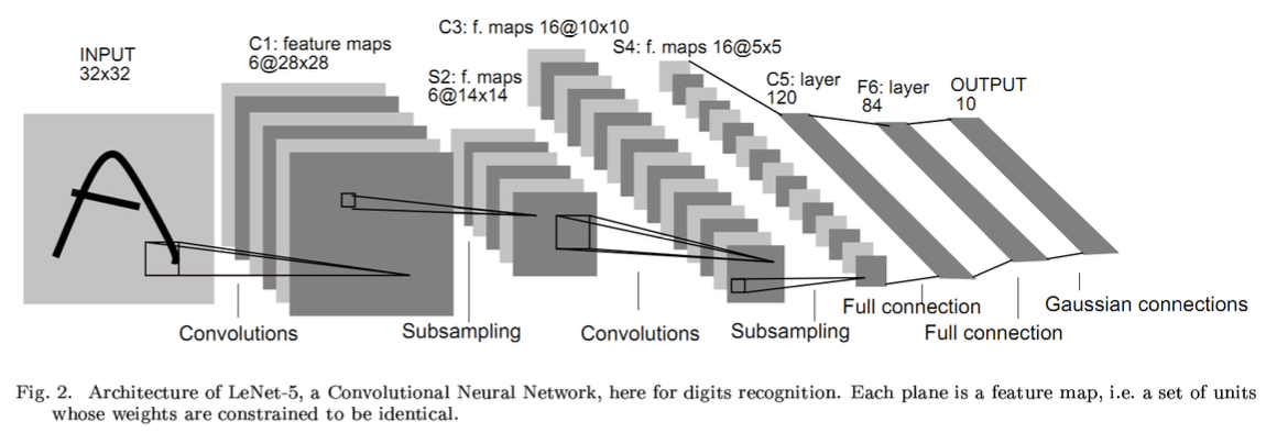
LeNet은 두 번의 convolution, pooling 을 거친 뒤, 2개의 fully connected layer 를 이용한다.
Feed-forward (fully connected) neural network 는 이미지 전체를 한 번에 인식한다.
ex) input(32,32,3) -> 3072로 flatten -> Wx -> output : 10
필터는 이미지를 슬라이딩하며, element-wise dot product를 수행한다. 필터는 원하는 색상만 보기도 하고, 이미지의 경계선만을 찾기도 한다. 이러한 필터는 학습하여 얻을 수도 있다. 필터를 통과한 output image를 activation map 이라 하는데, 각 필터가 활성화 되는 지점이 표시된 이미지이기 때문이다. 각 필터별로 여러개의 activation maps 을 쌓는다. 각 관점별로 이미지를 해석한 결과이다.
CNN은 다음의 요소로 구성되어 있다.
- Convolution
- filters : 몇개의 필터를 이용할 것인가? 각 필터의 크기는 어떻게 설정할 것인가?'
- stide : 필터를 몇 칸씩 움직일 것인가?
- padding : Activation map의 크기를 input image 와 일정하게 맞출 것인가?
- W'(activation map의 크기) = W(input image)-F(filter)+2P(padding)/S(stride) +1
- Subsampling
- Max-pooling
- Average pooling
- k-max pooling
- Activation : pooling을 거친 activation maps 의 값에 비선형성을 더해준다.(sigmoid, hyper-tangent, ReLU)
CNN은 여러 개의 관점(필터)로 이미지를 해석한 뒤, 유용한 정보만을 남겨(풀링) linear separable한 벡터(fully-connected)로 데이터의 representation을 변환한다.
from mnist_reader import load_mnist

train, train_labels = load_mnist(mnist_data_path, kind='train')
test, test_labels = load_mnist(mnist_data_path, kind='t10k') # fashion mnist data활용

print(train.shape) #(60000, 784)
print(train_labels.shape) #(60000,)

import numpy as np

image_samples = [np.rot90(xi.reshape(28,28),k=2) for xi in train[:16]] #90도로 2번 rotation, 16개만 샘플링하여 보여줌
label_samples = train_labels[:16]

from time import time
from sklearn.preprocessing import MinMaxScaler, StandardScaler
from sklearn.neural_network import MLPClassifier
from sklearn import metrics

def train_and_evaluate(model, scaler, X_train, y_train, X_test, y_test):
    # training
    t = time()
    X_train_scaled = scaler.fit_transform(X_train)
    model.fit(X_train_scaled, y_train)
    t = time() - t # 학습에 걸린 시간
    print(f'training time = {t:.3} secs. with n={X_train.shape[0]}')

    # test
    t = time()
    X_test_scaled = scaler.transform(X_test)
    y_test_pred = model.predict(X_test_scaled)
    t = time() - t
    print(f'test     time = {t:.3} secs. with n={X_test.shape[0]}\n')
    print(metrics.classification_report(y_test, y_test_pred))

    return model

model = MLPClassifier(
    hidden_layer_sizes = (200, 50),
    activation = 'relu',
    solver = 'adam', # 'sgd'
    warm_start = True, # 기존의 학습 이력 삭제?
    max_iter = 1000,
    epsilon = 0.00001
)

scaler = StandardScaler()

n_samples = 3000
X = train[:n_samples]
y = train_labels[:n_samples]

model = train_and_evaluate(model, scaler, X, y, test, test_labels)

print(f'num layers = {len(model.coefs_)}')

coefs = model.coefs_
intercepts = model.intercepts_

for l, (coef, intercept) in enumerate(zip(coefs, intercepts)):
    print(f'layer#{l+1}: coef={coef.shape}, intercept={intercept.shape}')


# num layers = 3
#layer#1: coef=(784, 200), intercept=(200,)
#layer#2: coef=(200, 50), intercept=(50,)
#layer#3: coef=(50, 10), intercept=(10,)
[코드 출처: lovit, 김현중 선생님의 깃허브 패스트캠퍼스 강의 발췌]
'센서 신호처리' 카테고리의 다른 글
| [논문 리뷰] A Road Condition Classification Algorithm for a Tire Acceleration Sensor using an Artificial Neural Network (0) | 2020.09.14 |
|---|---|
| [BLE] Nordic Enhanced ShockBurst User Guide (0) | 2020.09.12 |
| [머신러닝 6강] Preprocessing & Feature extraction (0) | 2020.08.30 |
| [머신러닝4강] Neural Network (0) | 2020.08.16 |
| [머신러닝 2강] Linear Regression (0) | 2020.08.08 |